The learning rate sets the lifetime of SGD's randomness
Pause a neural network training run at 60% of the way through training. Save weights, momentum buffers, remaining data, and the order of every future minibatch.
Now branch into two paths. One path is where you make the model consume the next two batches, namely and , in its original order. The other path is where you make the model consume the same two batches, but in reverse order, and . Continue as you would normally in both paths, i.e. onwards in the exact same order as the original run.
What would you expect to happen? Nothing? How would it affect the predictions of the model? Well, it depends.
With a learning rate of 0.05, that single intervention changes 33.6% of the final test predictions. Repeat from the same checkpoint with a learning rate of 0.005 and it changes only 0.2%.
Nothing about the model’s past changed. Nor its future data. The step size alone determines whether a, dare I say, random coin flip of the order of two batches disappears or grows into a different function altogether.
The result is obviously not that stochastic gradient descent is stochastic. It is that the learning rate sets the lifetime of that randomness.
A single controlled difference
Two training runs can differ in too many ways at once. Initializations, augmentations, and minibatch orders introduce countless independent perturbations. In turn, when trained models disagree, every randomness factor becomes a suspect.
This experiment leaves one suspect.
For every run, full minibatch order is fixed before training. Step of (count of all steps) consumes minibatch so the schedule is fixed in advance and never resampled.
At a chosen step, the training state is saved. Two branches continue:
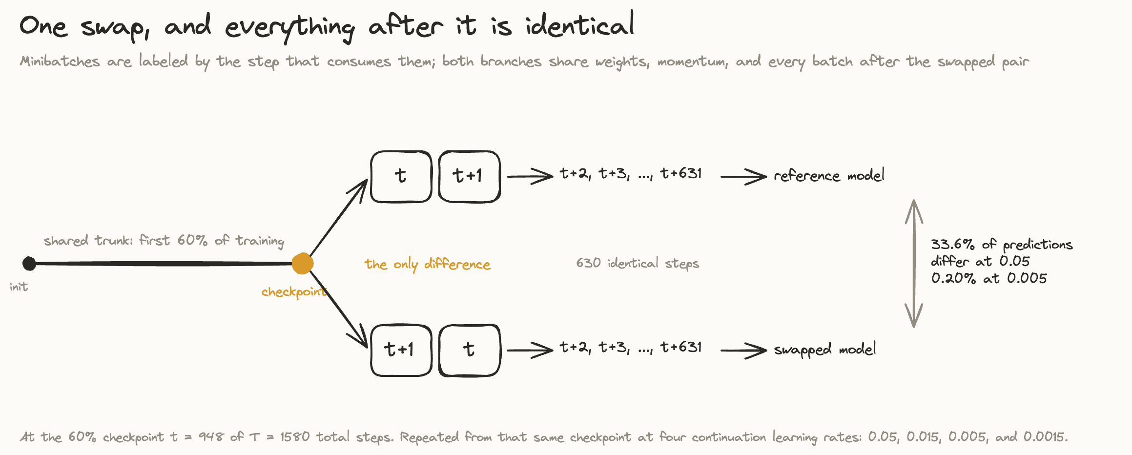
Both branches start from exactly identical weights and momentum, having consumed same batches up until the swap. After the swapped pair, every subsequent update is in sync. There is no random augmentation, crop, dropout, or batch normalization.
The two branches do not receive the same gradients in reverse order. A gradient depends on the parameters at which it is evaluated. Once has updated the model, sees a different model. Writing for the update that consumes , acting on the weights ,
Noncommutativity of these updates creates the difference as a natural consequence. The real question is what remaining updates do to it.
One early swap nearly matches a full reshuffle
The setup is intentionally plain. A small network with four convolutions, 10k subset of CIFAR-10, SGD with momentum 0.9 and weight decay 5e-4 on batches of 128, 3 different seeds. Training runs for 20 epochs ( steps) at a learning rate of 0.05 which drops to a tenth at epoch 12 (60%) and 17 (85%).
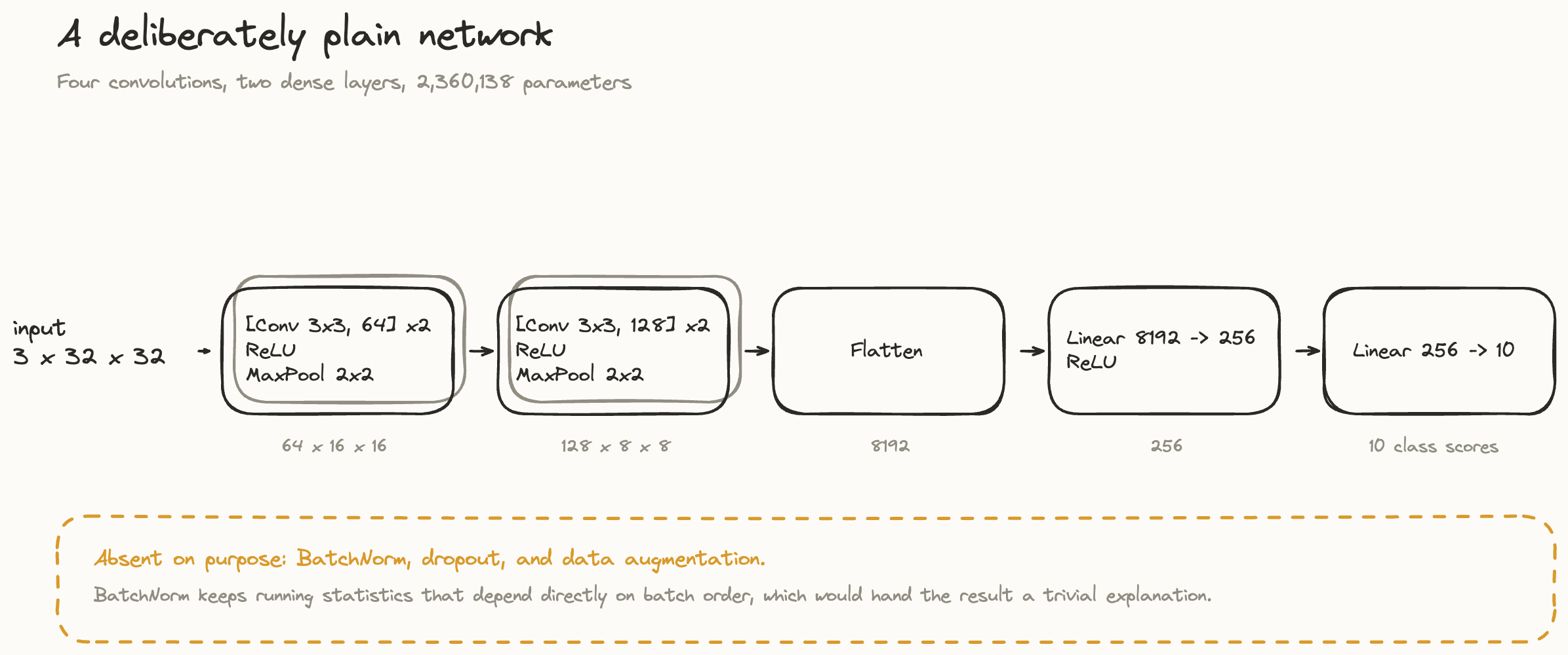
The absences matter more than the layers. BatchNorm keeps running statistics that update in batch order, so leaving it out removes the most boring explanation before I even start: any effect I see cannot be blamed on BatchNorm quietly reacting to the swap.
With that out of the way, I need to answer two separate questions. Did the decision change, and by how much did the model move over my fixed test set (5k images)?
More formally, over test images and classes, let be the logit vectors the two branches assign to image .
Define prediction disagreement as the fraction of images whose predicted class flips:
Define logit distance as the RMS gap across every logit:
Now the numbers. Two anchors first. Repeat the reference run from scratch ceteris paribus, on the same hardware (Apple MPS, PyTorch 2.6.0), and it lands bit-for-bit identical, and . That is the floor, and it is only to make sure the measurement has no hidden randomness. At the other extreme, throw away the batch order entirely and draw a fresh one, new permutations with new batch compositions: in seed 0 that changes 31.4% of predictions. Call it a rough ceiling, roughly the most disorder this simple setup can absorb.
The swap sits almost at that ceiling. Reversing just the first pair changes 30.7% of predictions in seed 0, and 29.8% averaged across the three seeds we have. One adjacent swap, held fixed forever after, does nearly the work of reshuffling all 1,580 steps.
Accuracy never sees it. The reference models average 63.5%; the swapped branches average 63.4%. The two are equally “good”. They just get different images right. That is the whole reason disagreement, not accuracy, is the metric that I think matters here. A scoreboard can read identical while the decisions underneath tell another story.
Swap persistence
Move the position the swap occurs at through training and its influence appears to have a lifetime.
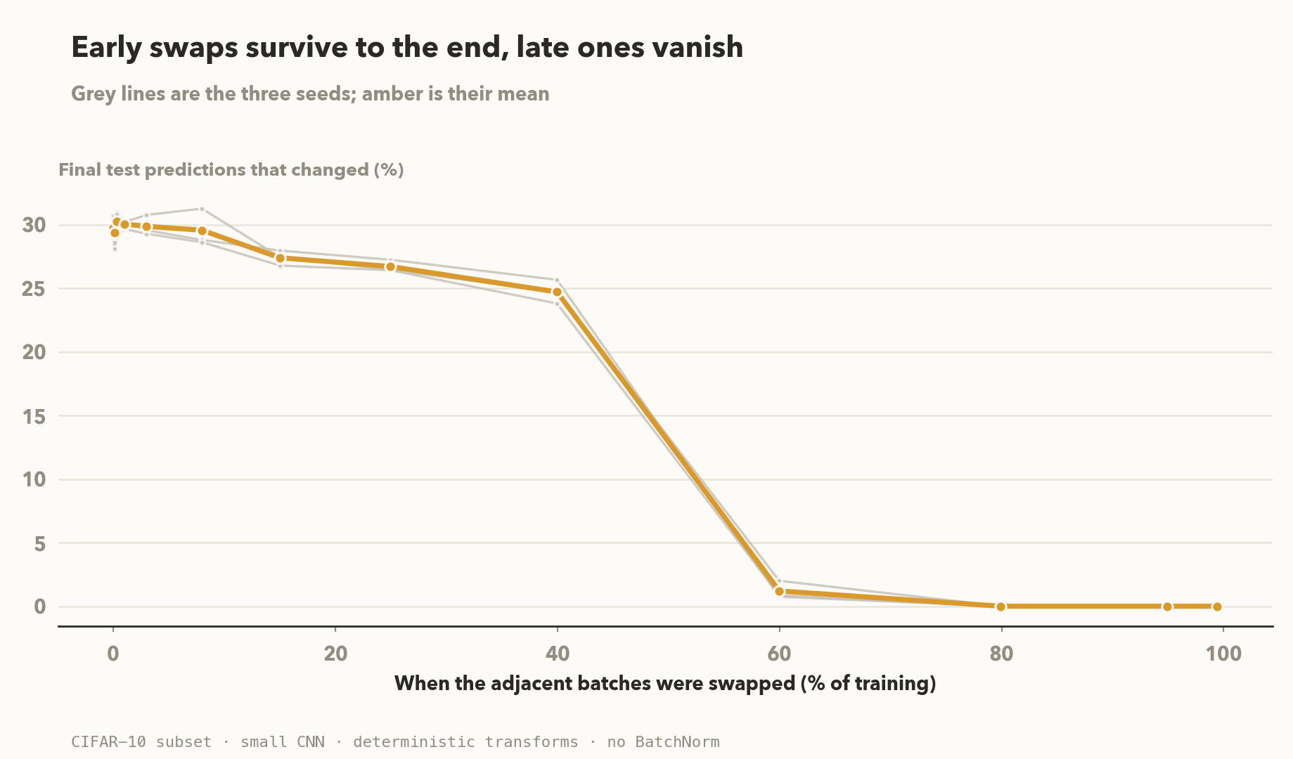
Initialization swap () changes 29.8% of final predictions. A swap at 40% () still changes 24.7%. Every swap in between executes at the same learning rate of 0.05, i.e. the gradual 5 pp decline is what training buys on its own.
Then the curve collapses to 1.2% at 60% and near-zero at 80%.
Should we be relieved? Early training chooses among possible solutions and later training refines over it. After enough updates the model becomes too settled for one slip?
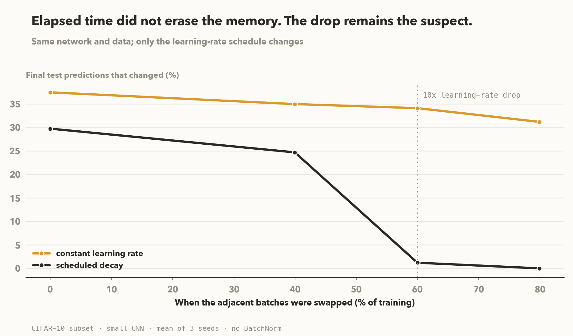
Our setup, unfortunately yields a rival. LR scheduled drop occurs at exactly 60% of training.
Elapsed time and step size move together in the first experiment and the curve cannot tell them apart. A control run clears the air. Hold the rate at 0.05 the whole way and the effect of the swap refuses to vanish.
A word on “memory”: the network is not storing the swap. High learning-rate steps keep amplifying the tiny difference the swap created, and low ones stop amplifying it. Memory here means an amplified perturbation still surviving, not information the model deliberately keeps.
Under the constant rate, a swap at 60% still changes 34.1% of final predictions, yet that control follows a different trajectory and lands at a lower accuracy of 59.8% against the original 63.5%. A cleaner test must change the learning rate without changing the checkpoint. Only then does suggestive evidence turn into a real claim.
The same past, four possible futures
The intervention I opened with, now in the controlled form the last section demanded. At the end of epoch 12, exactly 60% through training, I save one checkpoint per seed and let every branch start from that same frozen state. The past is now identical for all of them. The only thing I change going forward is the learning rate.
From each checkpoint I run four pairs: a reference and a swapped branch at four constant learning rates. All eight share the same history, the same momentum, and the same remaining batch sequence. Two things vary, and only two: whether and are swapped, and the size of every gradient step that follows.
The effect is not a slope. It is a cliff.
| Continuation learning rate | Final prediction disagreement (3-seed mean) |
|---|---|
| 0.0500 | 33.6% |
| 0.0150 | 2.3% |
| 0.0050 | 0.2% |
| 0.0015 | 0.08% |
Drop the rate tenfold, from 0.05 to 0.005, and the same swap goes from rewriting a third of the test predictions to two in a thousand. Same checkpoint, same swap, same future batches. Only the step size moved. The seeds barely argue about it: at 0.05 they span 33.4% to 33.7%, so this is a cliff, not a coincidence.
At 0.05 the swap even beats the full-reshuffle ceiling we derived earlier. In seed 0, reshuffling every batch changed 31.4% of predictions, yet one swap at 60% continued at 0.05 changes 33.7%. That is not a contradiction. The ceiling was measured under the decayed schedule, and a branch that keeps training at 0.05 never pays the decay, so one swap under the hotter rate can outrun a full reshuffle under the original recipe.
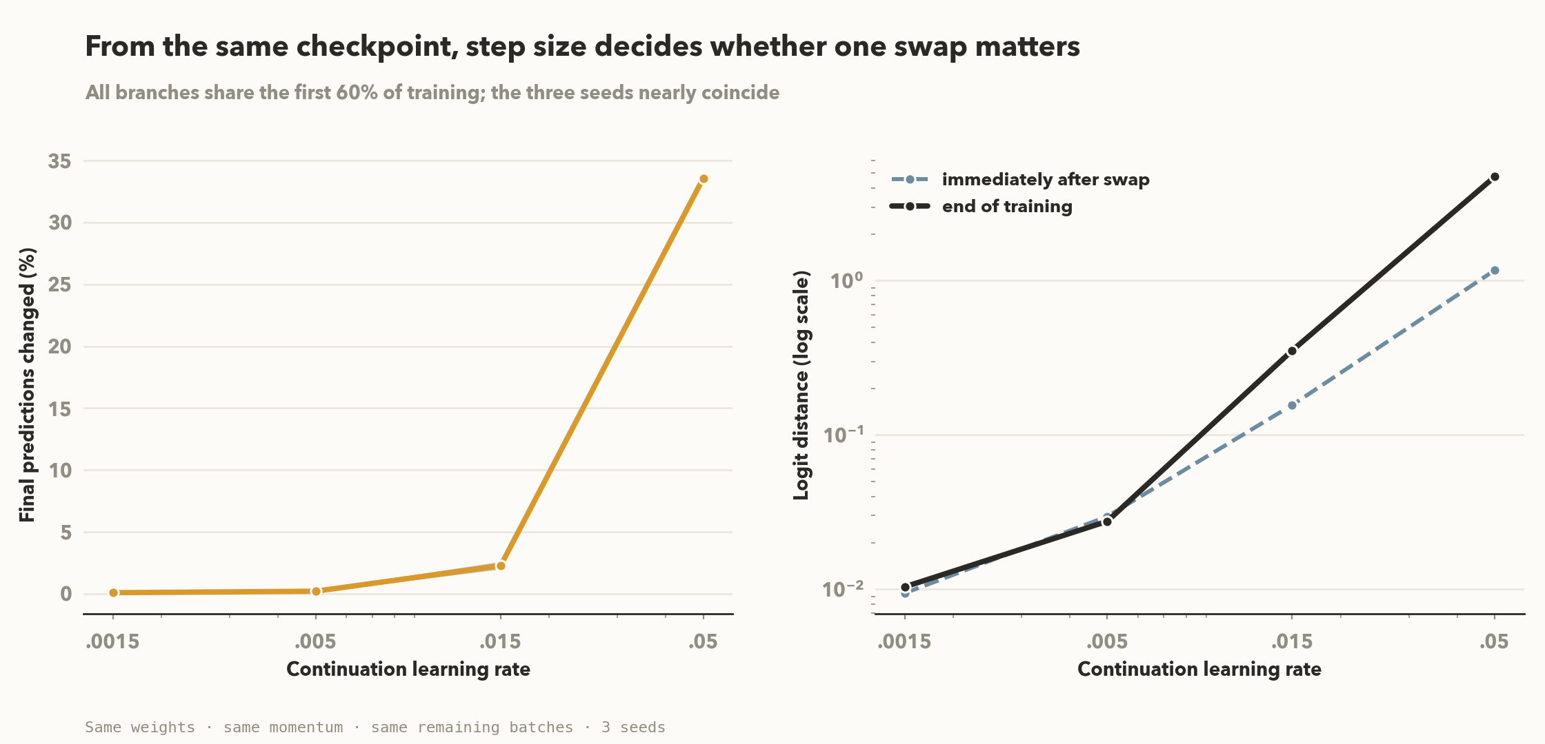
The right panel splits the effect in two. At 0.05 the swap opens a logit distance of 1.17 the moment it happens, and the remaining training grows it to 4.73. At 0.015 the kick (the difference the swap creates instantaneously) is smaller but still more than doubles, 0.16 to 0.35. At 0.005 the immediate and final distances are the same, 0.03 and 0.03, nothing grows. At 0.0015 both are essentially zero.
So step size acts twice. A high rate makes the initial ordering difference larger, then drops the model into dynamics that keep amplifying it. Lowering the rate shrinks the kick and, somewhere between 0.015 and 0.005, switches the amplification off.
That same split reconciles the two experiments. The persistence curve reported 1.2% for a swap at 60%, while this table reports 0.2% at 0.005, the rate the schedule decays to there. In the scheduled run the swap straddles the drop: its first swapped update still fires at 0.05, so the kick is an order of magnitude larger before the low rate takes over. In the checkpoint run, both swapped updates happen at the low rate from the start.
None of this makes 0.005 a universal safe rate. The number belongs to this network, this optimizer, this checkpoint, this data scale. The object that generalizes is the transition itself: as step size falls, the continuation moves from amplifying a perturbation to, well, just ignoring it.
What the decay is doing
Learning rate decay is conceptualized geometrically. Smaller steps refine without bouncing around while larger steps make rapid progress. With one-swap experiment we get a story of functional consequence.
Pre-decay, training is sensitive to details. A single sequence change amplifies itself until a third of the decision function outcomes change. After the decay, later updates do not turn the model into a different classifier.
It is stronger than saying small updates produce small changes. We show that at the high rate the perturbation not only persists but grows: the final difference exceeds the immediate one. Around the decayed rate it does neither. The kick lands, and then the remaining training carries it along unchanged rather than building on it.
That is the whole point. It is not that the same process runs slower at a lower rate. It is that the process is different. One rate turns a two-batch accident into a different classifier; the other lets it sit where it fell and forgets to make anything of it. The decay does not just shrink the steps. It ends the regime that could amplify.
What to do about it
If individual predictions matter (which they usually do), performance metrics alone cannot tell you a recipe is stable. Two models can score the same and still disagree on a third of the cases, as shown. The usual reproducibility advice applies. What this experiment adds is a single lever on top of it: the learning rate decides how much of that randomness survives into the final model.
- Treat the final learning rate as a decision-stability control. Hold it high to the end and one reshuffle-sized accident can still rewrite a third of your predictions. A low-rate finish stops training from amplifying that accidental history. Before export, continue at a lower rate and check whether disagreement across retrains falls without costing accuracy you need. One small CNN is not a universal recipe.
- The usual discipline still holds underneath it. Enumerate your sources of randomness: initialization, augmentations, batch order, dropout, nondeterministic kernels. Measure pairwise disagreement across retrains rather than accuracy alone, and slice it where a flipped decision is costly. And do not mistake a fixed seed for reproducible decisions, since order and hardware nondeterminism still cascade into a different model.
The distinction underneath both:
Watch only the metric and the instability stays invisible.
Limitations and prior work
None of the ingredients are new. Theory already ties step size to how much one changed example moves SGD’s output (Hardt et al., 2016), whether a perturbation grows or dies is a linear-stability question, the same boundary that full-batch training drifts toward as the edge of stability (Cohen et al., 2021), run-to-run prediction differences are well documented down to a single flipped bit (Summers & Dinneen, 2021; Jiang et al., 2022), networks stabilize against SGD noise over training (Frankle et al., 2020), batch order can even be an attack (Shumailov et al., 2021), and shuffling interacts with BatchNorm (Wu et al., 2023), which is why it is absent here. What this post adds is one concrete demonstration: a single adjacent swap held fixed, and the same checkpoint continued at four rates.
The model is deliberately weak, 63.5% on a small unaugmented CIFAR-10 subset, so the specific threshold does not transfer to a modern recipe. A weak model probably makes the effect easy to see: near 63% accuracy, many predictions sit close to a decision boundary, where a small nudge flips them. Whether a stronger recipe damps this or just hides it behind a better average is exactly what this experiment cannot say. I do not show the branches sit in different basins or that either is better, and momentum is part of the mechanism rather than a controlled variable. The high-rate branches are also less accurate, so the sensitivity may be a symptom of training near instability rather than a virtue of SGD.
The narrow result survives all of that: from identical training state, a tenfold change in learning rate moves one adjacent swap from changing a third of the predictions to two in a thousand. The data does not fix one inevitable classifier; the learning rate helps decide which accidents you ship.
References
Cohen, J. M., Kaur, S., Li, Y., Kolter, J. Z., & Talwalkar, A. (2021). Gradient descent on neural networks typically occurs at the edge of stability. International Conference on Learning Representations (ICLR). https://doi.org/10.48550/arXiv.2103.00065
Frankle, J., Dziugaite, G. K., Roy, D. M., & Carbin, M. (2020). Linear mode connectivity and the lottery ticket hypothesis. Proceedings of the 37th International Conference on Machine Learning (ICML). https://doi.org/10.48550/arXiv.1912.05671
Hardt, M., Recht, B., & Singer, Y. (2016). Train faster, generalize better: Stability of stochastic gradient descent. Proceedings of the 33rd International Conference on Machine Learning (ICML). https://doi.org/10.48550/arXiv.1509.01240
Jiang, Y., Nagarajan, V., Baek, C., & Kolter, J. Z. (2022). Assessing generalization of SGD via disagreement. International Conference on Learning Representations (ICLR). https://doi.org/10.48550/arXiv.2106.13799
Shumailov, I., Shumaylov, Z., Kazhdan, D., Zhao, Y., Papernot, N., Erdogdu, M. A., & Anderson, R. J. (2021). Manipulating SGD with data ordering attacks. Advances in Neural Information Processing Systems 34 (NeurIPS). https://doi.org/10.48550/arXiv.2104.09667
Summers, C., & Dinneen, M. J. (2021). Nondeterminism and instability in neural network optimization. Proceedings of the 38th International Conference on Machine Learning (ICML). https://doi.org/10.48550/arXiv.2103.04514
Wu, D. X., Yun, C., & Sra, S. (2023). On the training instability of shuffling SGD with batch normalization. Proceedings of the 40th International Conference on Machine Learning (ICML). https://doi.org/10.48550/arXiv.2302.12444